🧑‍🏫 Lecture 3

Pruning and Sparsity (Part I)

앞으로 총 5장에 걸쳐서 딥러닝 모델 경량화 기법들에 대해서 소개하려고 한다. 경량화 기법으로는 Pruning, Quantization, Neural Network Architecture Search, Knowledge Distillation, 그리고 Tiny Engine에서 돌리기 위한 방법을 진행할 예정인데 본 내용은 MIT에서 Song Han 교수님이 Fall 2022에 한 강의 TinyML and Efficient Deep Learning Computing 6.S965를 바탕으로 재정리한 내용이다. 강의 자료와 영상은 이 링크를 참조하자!

첫 번째 내용으로 “가지치기”라는 의미를 가진 Pruning에 대해서 이야기, 시작!

1. Introduction to Pruning

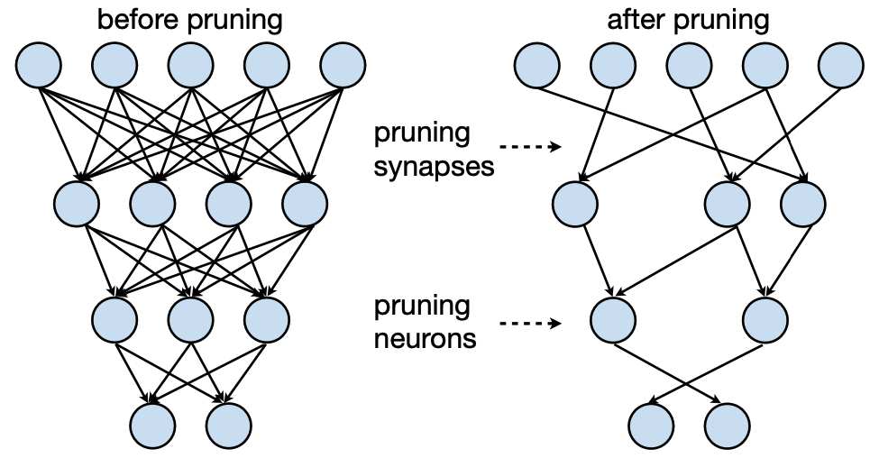
Pruning이란 의미처럼 Neural Network에서 매개변수(노드)를 제거하는 방법입니다. 이는 Dropout하고 비슷한 의미로 볼 수 있는데, Dropout의 경우 모델 훈련 도중 랜덤적으로 특정 노드를 제외시키고 훈련시켜 모델의 Robustness를 높이는 방법으로 훈련을 하고나서도 모델의 노드는 그대로 유지가 된다. 반면 Pruning의 경우 훈련을 마친 후에, 특정 Threshold 이하의 매개변수(노드)의 경우 시 Neural Network에서 제외시켜 모델의 크기를 줄이면서 동시에 추론 속도 또한 높일 수 있다.

\[ \underset{W_p}{argmin}\ L(x;W_p), \text{ subject to } \lvert\lvert W_p\lvert\lvert_0\ < N \]

• L represents the objective function for neural network training
• \(x\) is input, \(W\) is original weights, \(W_p\) is pruned weights
• \(\lvert\lvert W_p\lvert\lvert_0\) calcuates the #nonzeros in \(W_p\) and \(N\) is the target #nonzeros

이는 위와 같은 식으로 표현할 수 있다. 특정 W 의 경우 0 으로 만들어 노드를 없애는 경우라고 볼 수 있겠습니다. 그렇게 Pruning한 Neural Network는 아래 그림 처럼 된다.

Reference. MIT-TinyML-lecture03-Pruning-1

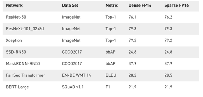
그럼 왜 Pruning을 하는 걸까? 강의에서 Pruning을 사용하면 Latency, Memeory와 같은 리소스를 확보할 수 있다고 관련된 아래같은 연구결과를 같이 보여준다.

Reference. MIT-TinyML-lecture03-Pruning-1

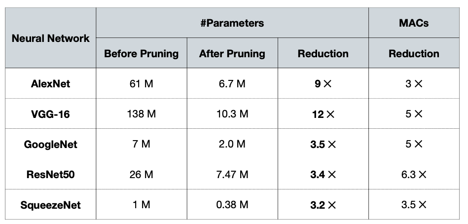
Song Han 교수님은 Vision 딥러닝 모델 경량화 연구를 주로하셔서, CNN을 기반으로 한 모델을 예시로 보여주신다. 모두 Pruning이후에 모델 사이즈의 경우 최대 12배 줄어 들며 연산의 경우 6.3배까지 줄어 든 것을 볼 수 다.

그렇다면 저렇게 “크기가 줄어든 모델이 성능을 유지할 수 있을까?“

Reference. MIT-TinyML-lecture03-Pruning-1

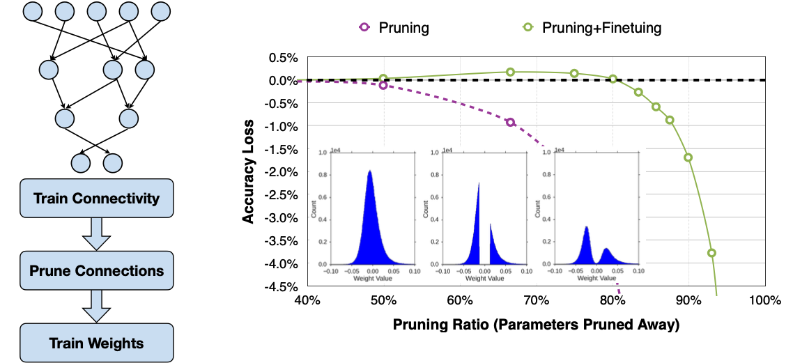
그래프에서 모델의 Weight 분포도를 위 그림에서 보면, Pruning을 하고 난 이후에 Weight 분포도의 중심에 파라미터가 잘려나간 게 보인다. 이후 Fine Tuning을 하고 난 다음의 분포가 나와 있는데, 어느 정도 정확도는 떨어지지만 성능이 유지되는 걸 관찰할 수 있다.

Reference. MIT-TinyML-lecture03-Pruning-1

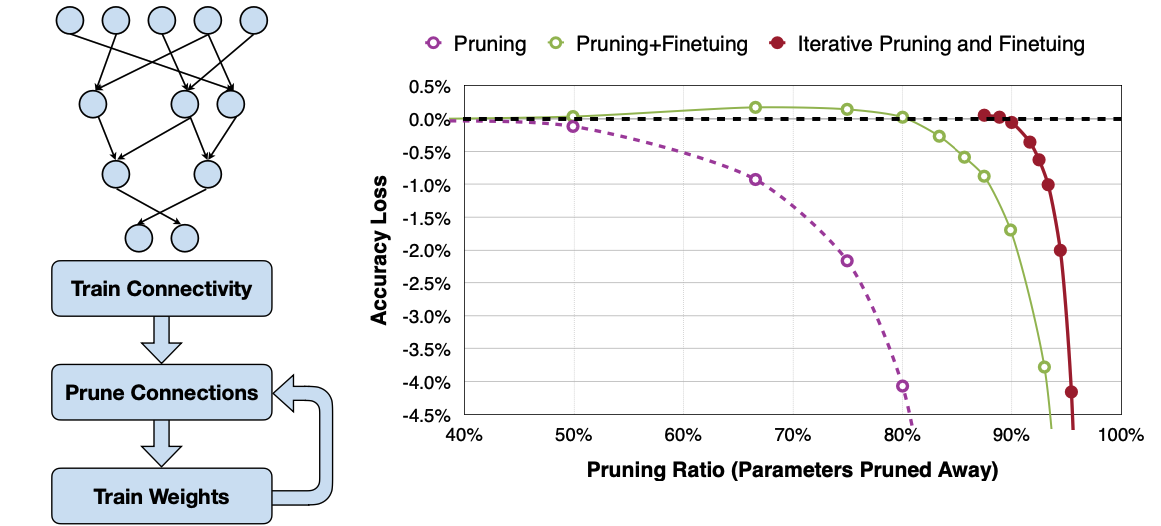
그런 Fine tuning을 반복적으로 하게 된다면(Iterative Pruning and Fine tuning) 그래프에서는 최대 90프로 이상의 파라미터를 덜어낼 수 있다고 한다.

물론 특정 모델에서, 특정 Task를 대상으로 한 것이라 일반화할 수는 없지만 리소스를 고려하는 상황이라면 충분히 시도해볼 만한 가치가 있어 보인다. 그럼 이렇게 성능을 유지하면서 Pruning을 하기 위해서 어떤 요소를 고려해야 할지 더 자세히 이야기해보자!

소개하는 고려요소는 아래와 같다. Pruning 패턴부터 차례대로 시작!

• Pruning Granularity → Pruning 패턴
• Pruning Criterion → 얼마만큼에 파라미터를 Pruning 할 건가?
• Pruning Ratio → 전체 파라미터에서 Pruning을 얼마만큼의 비율로?
• Fine Turning → Pruning 이후에 어떻게 Fine-Tuning 할 건가?
• ADMM → Pruning 이후, 어떻게 Convex가 된다고 할 수 있지?
• Lottery Ticket Hypothesis → Training부터 Pruning까지 모델을 만들어 보자!
• System Support → 하드웨어나 소프트웨어적으로 Pruning을 지원하는 경우는?

2. Determine the Pruning Granularity

The case of convolutional layers, red box is preserved and white one is pruned referred from MIT-TinyML-lecture03-Pruning-1

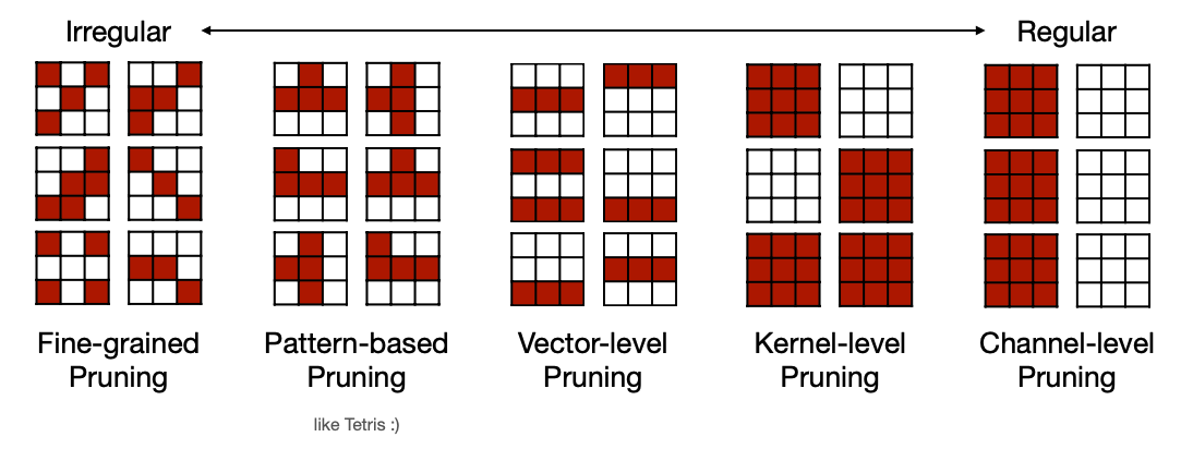
여기서 고려요소는 “얼마만큼 뉴런을 그룹화하여 고려할 것인가?” 입니다. Regular한 정로도 분류하면서 Irregular한 경우와 Regular한 경우의 특징을 아래처럼 말합니다.

• Fine-grained/Unstructured
  • More flexible pruning index choice
  • Hard to accelerate (irregular data expression)
  • Can deliver speed up on some custom hardware
• Coarse-grained/Structured
  • Less flexible pruning index choice (a subset of the fine-grained case)
  • Easy to accelerate

Pruning을 한다고 모델 출력이 나오는 시간이 짧아지는 것이 아님도 언급합니다. Hardware Acceleration의 가능도가 있는데, 이 특징을 보면 알 수 있듯, Pruning의 자유도와 Hardware Acceleration이 trade-off, 즉 경량화 정도와 Latency사이에 trade-off 가 있을 것이 예측됩니다. 하나씩, 자료를 보면서 살펴 보겠습니다.

2.1 Pattern-based Pruning

Irregular에서도 Pattern-based Pruning은 연속적인 뉴런 M개 중 N개를 Pruning 하는 방법이다. 일반적으로는 N:M = 2:4 으로 한다고 소개한다.

Reference. Accelerating Inference with Sparsity Using the NVIDIA Ampere Architecture and NVIDIA TensorRT

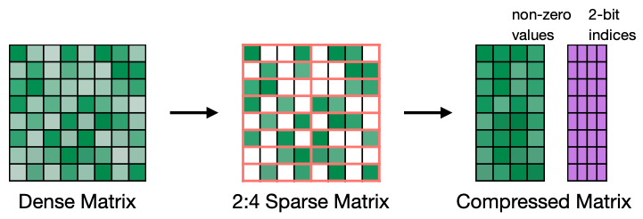
Reference. Accelerating Inference with Sparsity Using the NVIDIA Ampere Architecture and NVIDIA TensorRT

예시를 들어 보면, 위와 같은 Matrix에서 행을 보시면 8개의 Weight중 4개가 Non-zero인 것을 볼 수 있습니다. 여기서 Zero인 부분을 없애고 2bit index로 하여 Matrix 연산을 하면 Nvidia’s Ampere GPU에서 속도를 2배까지 높일 수 있다고 한다. 여기서 Sparsity는 “얼마만큼 경량화 됐는지?” 이라고 생각하면 된다.

• N:M sparsity means that in each contiguous M elements, N of them is pruned
• A classic case is 2:4 sparsity (50% sparsity)
• It is supported by Nvidia’s Ampere GPU Architecture, which delivers up to 2x speed up and usually maintains accuracy.

Reference. https://developer.nvidia.com/blog/accelerating-inference-with-sparsity-using-ampere-and-tensorrt/

2.2 Channel-level Pruning

반대로 패턴이 상대적으로 regular 한 쪽인 Channel-level Pruning은 추론시간을 줄일 수 있는 반면에 경량화 비율이 적다고 말한다. 아래 그림을 보시면 Layer마다 Sparsity가 다른 걸 보실 수 있다.

• Pro: Direct speed up!
• Con: smaller compression ratio

Reference AMC: Automl for Model Compression and Acceleration on Mobile Devices [He et al., ECCV 2018]

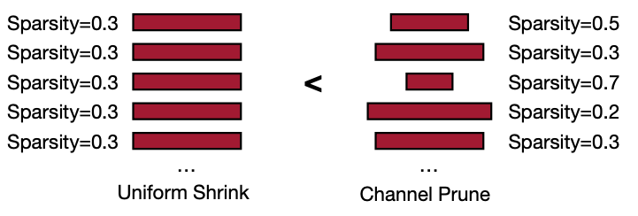
아래에 자료에서는 Channel 별로 한 Pruning의 경우 전체 뉴련을 가지고 한 Pruning보다 추론 시간을 더 줄일 수 있다고 말한다.

Reference AMC: Automl for Model Compression and Acceleration on Mobile Devices [He et al., ECCV 2018]

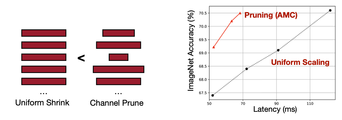
자료를 보면 Sparsity에서는 패턴화 돼 있으면 가속화가 용이해 Latency, 추론 시간을 줄일 수 있지만 그 만큼 Pruning하는 뉴런의 수가 적어 경량화 비율이 줄 것으로 보인다. 하지만 비교적 불규칙한 쪽에 속하는 Pattern-based Pruning의 경우가 하드웨어에서 지원해주는 경우, 모델 크기와 Latency를 둘 다 최적으로 잡을 수 있을 것으로 보인다.

3. Determine the Pruning Criterion

그렇다면 어떤 파라미터를 가지는 뉴런을 우리는 잘라내야 할까요? Synapse와 Neuron으로 나눠서 살펴보자.

• Which synapses? Which neurons? Which one is less important?
• How to Select Synapses and Select Neurons to Prune

3.1 Select of Synapses

크게 세 가지로 분류하는데, 각 뉴런의 크기, 각 채널에 전체 뉴런에 대한 크기, 그리고 테일러 급수를 이용하여 gradient와 weight를 모두 고려한 크기를 소개한다. Song han 교수님이 방법들을 소개하기에 앞서서 유수의 기업들도 지난 5년 동안 주로 Magnitude-based Pruning만을 사용해왔다고 하는데, 2023년이 돼서 On-device AI가 각광받기 시작해서 점차적으로 관심을 받기 시작한 건가 싶기도 하다.

3.1.1 Magnitude-based Pruning

크기를 기준으로 하는 경우, “얼마만큼 뉴런 그룹에서 고려할 것인가?”와 “그룹내에서 어떤 정규화를 사용할 것인가?를 고려한다.

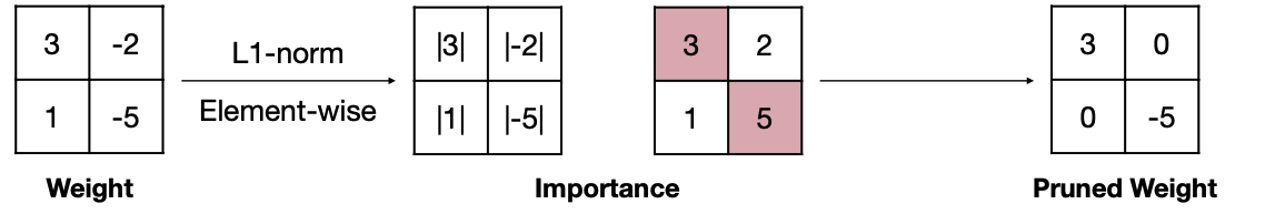
1. Heuristic pruning criterion, Element-wise Pruning

   \[ Importance = \lvert W \lvert \]

   

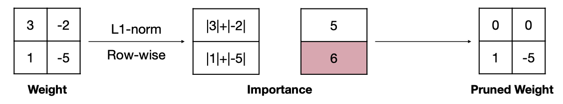
   Reference. MIT-TinyML-lecture03-Pruning-1

2. Heuristic pruning criterion, Row-wise Pruning, L1-norm magnitude

   \[ Importance = \sum_{i\in S}\lvert w_i \lvert, \\where\ W^{(S)}\ is\ the\ structural\ set\ S\ of\ parameters\ W \]

   

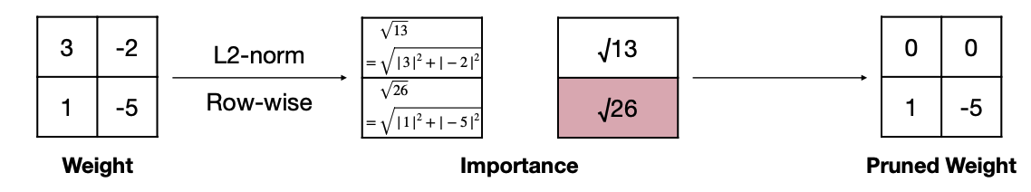
   Reference. MIT-TinyML-lecture03-Pruning-1

3. Heuristic pruning criterion, Row-wise Pruning, L2-norm magnitude

   \[ Importance = \sum_{i\in S}\lvert w_i \lvert, \\where\ W^{(S)}\ is\ the\ structural\ set\ S\ of\ parameters\ W \]

   

   Reference. MIT-TinyML-lecture03-Pruning-1

4. Heuristic pruning criterion, \(L_p\)- norm

   \[ \lvert\lvert W^{(S)}\lvert\lvert=\huge( \large \sum_{i\in S} \lvert w_i \lvert^p \huge) \large^{\frac{1}{p}} \]

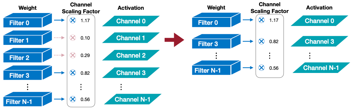
3.1.2 Scaling-based Pruning

두 번째로 Scaling을 하는 경우 채널마다 Scaling Factor를 둬서 Pruning을 한다. 그럼 Scaling Factor를 어떻게 둬야 할까? 강의에서 소개하는 이 논문에서는 Scaling factor \(\gamma\) 파라미터를 trainable 파라미터로 두면서 batch normalization layer에 사용한다.

• Scale factor is associated with each filter(i.e. output channel) in convolution layers.

• The filters or output channels with small scaling factor magnitude will be pruned

• The scaling factors can be reused from batch normalization layer

  \[ z_o = \gamma\dfrac{z_i-\mu_{B}}{\sqrt{\sigma_B^2+\epsilon}}+\beta \]

Reference. MIT-TinyML-lecture03-Pruning-1

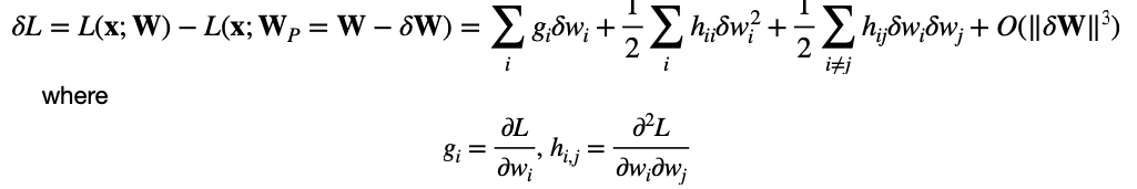
3.1.3 Talyor Expansion Analysis on Pruning Error

세 번째 방법은 테일러 급수를 이용하여 Objective function을 최소화 하는 지점을 찾는 방법입니다. Talyor Series에 대한 자세한 내용은 여기서!

• Evaluate pruning error induced by pruning synapses.
• Minimize the objective function L(x; W)
• A Taylor series can approximate the induced error.

\[ \delta L = L(x;W)-L(x;W_p=W-\delta W) \\ = \sum_i g_i\delta w_i + \frac{1}{2} \sum_i h_{ii}\delta w_i^2 + \frac{1}{2}\sum_{i\not=j}h_{ij}\delta w_i \delta w_j + O(\lvert\lvert \delta W \lvert\lvert^3) \] \[ where\ g_i=\dfrac{\delta L}{\delta w_i}, h_{i, j} = \dfrac{\delta^2 L}{\delta w_i \delta w_j} \]

1. Second-Order-based Pruning

   

   Reference. MIT-TinyML-lecture03-Pruning-1

   

   Reference. MIT-TinyML-lecture03-Pruning-1

   Optimal Brain Damage[LeCun et al., NeurIPS 1989] 논문에서는 이 방법을 이용하기 위해 세 가지를 가정한다.

   1. Objective function L이 quadratic 이기 때문에 마지막 항이 무시된다(이는 Talyor Series의 Error 항을 알면 이해가 더 쉽다!)
   2. 만약 신경망이 수렴하게되면, 첫 번째항도 무시된다.
   3. 각 파라미터가 독립적이라면 Cross-term도 무시된다.

   그러면 식을 아래처럼 정리할 수 있는데, 중요한 부분은 Hessian Matrix H에 사용하는 Computation이 어렵다는 점!

   \[ \delta L_i = L(x;W)-L(x;W_p\lvert w_i=0)\approx \dfrac{1}{2} h_{ii}w_i^2,\ where\ h_{ii}=\dfrac{\partial^2 L}{\partial w_i \partial w_j} \]

   \[ importance_{w_i} = \lvert \delta L_i\lvert = \frac{1}{2}h_{ii}w_i^2 \] \[ *\ h_{ii} \text{ is non-negative} \]

2. First-Order-based Pruning

   • 참고로 이 방법은 2023년에는 소개하지 않는다.

   

   Reference. MIT-TinyML-lecture03-Pruning-1

   • If only first-order expansion is considered under an i.i.d(Independent and identically distributed) assumption,

   \[ \delta L_i = L(x;W) - L(x; W_P\lvert w_i=0) \approx g_iw_i,\ where\ g_i=\dfrac{\partial L}{\partial w_i} \] \[ importance_{w_i} = \lvert \delta L_i \lvert = \lvert g_i w_i \lvert \ or \ importance_{w_i} = \lvert \delta L_i \lvert^2 = (g_i w_i)^2 \]

   • For coarse-grained pruning, we have,

     \[ importance_{\ W^{(S)}} = \sum_{i \in S}\lvert \delta L_i \lvert^2 = \sum_{i \in S} (g_i w_i)^2,\ where \ W^{(S)}is\ the\ structural\ set\ of\ parameters \]

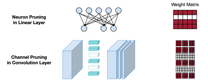
3.2 Select of Neurons

어떤 Neuron을 없앨 지를 고려(Less useful → Remove) 한 이 방법은 Neuron의 경우도 있지만 아래 그림처럼 Channel로 고려할 수도 있다. 확실히 전에 소개했던 방법들보다 “Coarse-grained pruning”인 방법이다.

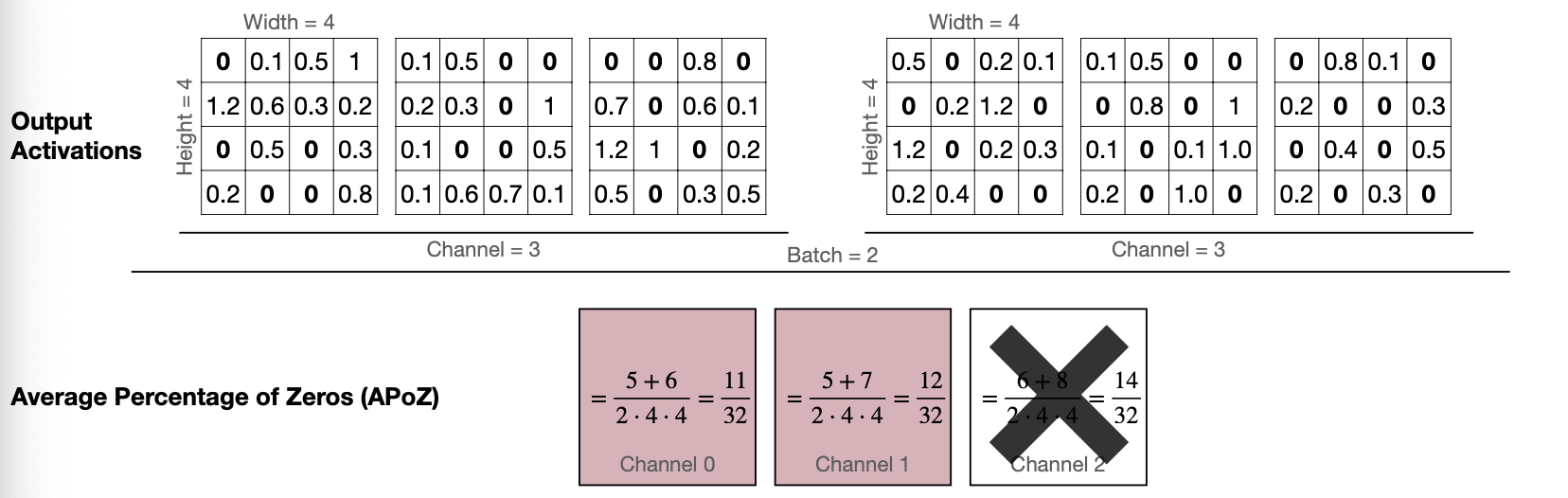
1. Percentage-of-Zero-based Pruning

   첫번째는 Channel마다 0의 비율을 봐서 비율이 높은 Channel 을 없내는 방법이다. ReLU activation을 사용하면 Output이 0이 나오는데, 여기서 0의 비율, Average Percentage of Zero activations(APoZ)라고 부르는 것을 보고 가지치기할 Channel을 제거한다.

   • ReLU activation will generate zeros in the output activation
   • Similar to magnitude of weights, the Average Percentage of Zero activations(APoZ) can be exploited to measure the importance the neuron has

   

   Reference. MIT-TinyML-lecture03-Pruning-1

2. First-Order-based Pruning

   • 참고로 이 방법은 2023년에는 소개하지 않는 방법이다.

   • Minimize the error on loss function introduced by pruning neurons

   • Similar to previous Taylor expansion on weights, the induced error of the objective function L(x; W) can be approximated by a Taylor series expanded on activations.

     \[ \delta L_i = L(x; W) - L(x\lvert x_i = 0; W) \approx \dfrac{\partial L}{\partial x_i}x_i \]

   • For a structural set of neurons \(x^{(S)}\) (e.g., a channel plane),

     \[ \lvert \delta L_{x^{(S)}} \lvert\ = \Large\lvert \small\sum_{i\in S}\dfrac{\partial L}{\partial x_i}x_i\Large\lvert \]

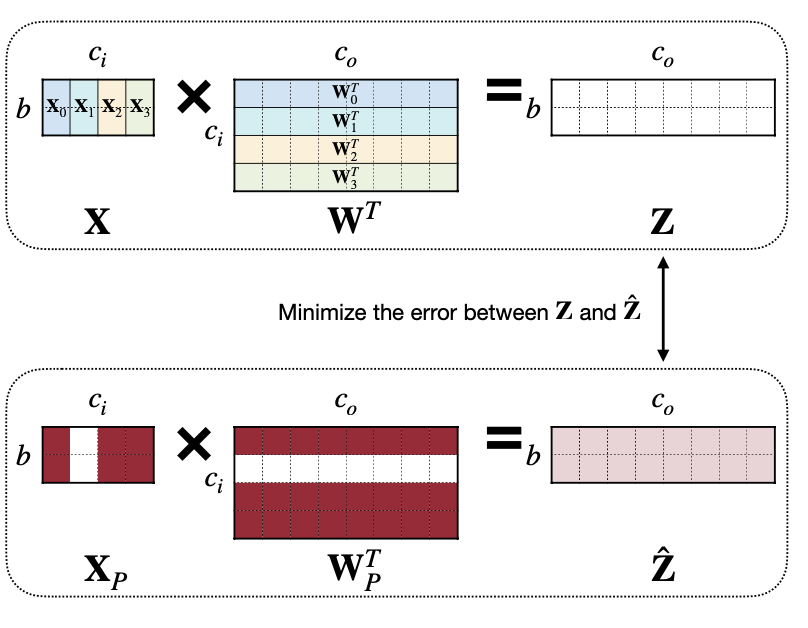
3. Regression-based Pruning

   이 방법은 Quantized한 레이어의 output \(\hat Z\)(construction error of the corresponding layer’s outputs)와 \(Z\)를 Training을 통해 차이를 줄이는 방법이다. 참고로 문제를 푸는 자세한 과정은 2022년 강의에만 나와 있다.

\[ Z=XW^T=\sum_{c=0}^{c_i-1}X_cW_c^T \]

Reference. MIT-TinyML-lecture03-Pruning-1

문제를 식으로 정의해보면 아래와 같은데,

• \(\beta\) is the coefficient vector of length \(c_i\) for channel selection.
• \(\beta_c = 0\) means channel \(c\) is pruned.
• \(N_c\) is the number of none zero channel

우선 문제를 푸는 단계는 두 단계로 나눈다. Channel의 Scale \(\beta\)를 우선 계산한 후에 \(W\)를 Quantized한 레이어의 output \(\hat Z\)(construction error of the corresponding layer’s outputs)와 \(Z\)의 차이가 최소화되는 지점까지 Training시킨다.

Solve the problem in two folds:

• Fix W, solve \(\beta\) for channel selection → NP(Nondeterministic polynomial)-hard
• Fix \(\beta\), solve W to minimize reconstruction error(Weight Reconstruction)

각 문제를 푸는 과정을 조금 더 자세히 살펴봐보자. 본 내용은 2022년 강의에 있으니 참고!

NP(Nondeterministic polynomial)-hard는 아래와 같이 식으로 정리할 수 있다.

\[ \underset{\beta}{argmin} \lvert\lvert Z- \sum_{c=0}^{c_i-1} \beta_cX_cW_c^T \lvert\lvert_F^2 = \lvert\lvert \sum_{c=0}^{c_i-1}X_cW_c^T - \sum_{c=0}^{c_i-1} \beta_cX_cW_c^T \lvert\lvert_F^2 \] \[ = \lvert\lvert\sum_{c=0}^{c_i-1} (1-\beta_c)X_cW_c^T \lvert\lvert_F^2, \ s.t.\ \lvert\lvert\beta\lvert\lvert_0 \ \leq N_c \]

강의에서 소개하는 ThiNet이라는 논문에서는 greedy solution을 이용해서 채널 하나하나씩 Pruning 해보며 objective function의 l2-norm 최솟값을 구한다.

1: S = []
2: while len(S) < N:
3:   min_norm, min_c = +inf, 0
4:   for c in range(c_i):
5:     tmpS=S+[c]
6:     Z = X[:,tmpS] * W[:,tmpS].t()
7:     norm = Z.norm(2)
8:     if norm < min_norm:
9:       min_norm, min_c = norm, c
10:   S.append(min_c)
11:   c_i.pop(min_c)

여기서 더해서 \(\beta\) 를 구하는 과정에서 일반화를 위해 LASSO 방식을 사용한다(LASSO에 대한 자세한 내용은 여기서). Relax the \(l_0\) to \(l_1\) regularization (LASSO):

\[ \underset{\beta}{argmin}\ \lvert\lvert Z- \sum_{c=0}^{c_i-1}\beta_cX_cW_c^T\lvert\lvert^2_F+\lambda\lvert\lvert \beta \lvert\lvert_1 \]

• \(\lambda\) is a penalty coefficient. By increasing \(\lambda\), there will be more zeros in \(\beta\).

• Gradually increase \(\lambda\) and solve the LASSO regression for \(\beta\), until \(\lvert\lvert \beta \lvert\lvert_0==N_c\) is met.

• Why \(\lvert\lvert \beta \lvert\lvert_0==N_c\)?

  여기에 대해서는 따로 언급되지 않았지만, 의미상 scale 전체 N개 중에서 최적값을 찾아야한다면 전체를 N으로 유지하면서 최적값을 찾기 위해서가 아닐까?

두 번째는 구한 \(\beta\)를 고정한 상태로 Weight를 Quantized 전후의 차이를 최소화 하게 “Weight Reconstruction” 한다. 구하는 과정은 least square approach를 이용한 unique closed-form solution 이므로 아래를 참조하자.

\[ \underset{\beta}{argmin}\ \lvert\lvert Z- \sum_{c=0}^{c_i-1}\beta_cX_cW_c^T\lvert\lvert^2_F \]

• \(\beta\) is a coefficient vector from the previous step

• This is a classic linear regression problem, which has a unique closed-form solution using the least square approach.

  \[ \underset{W}{argmin} \lvert\lvert Z-\hat{Z} \lvert\lvert^2_F = \lvert\lvert Z-UW^T \lvert\lvert_F^2 \]

  where

  \[ U= \Large[ \small\beta_0X_0\ \beta_1X_1 \ \cdots \beta_cX_c \cdots \beta_{c_i-1}X_{c_i-1} \Large] \]

  and thus,

  \[ W^T = (U^TU)^{-1}U^T Z \]

  • Q. How \((U^TU)^{-1}\) exists?

    Least Square method, 임의의 벡터 \(v = (v_0, v_1, \dots, v_n)\) 가 있을 때 \(v^Tv\) 의 역행렬은 항상 있을까? 가정에서 “a unique closed-form solution”라고 했으므로 이는 즉 linearly independen로 고려할 있고 역행렬이 있다(\(v^Tv\) is invertible)는 이야기이다.

4. Discussion

1. Pruning을 Dropout이랑 비교해서 어떤 차이점이 있는가?

   두 가지 방법은 분명히 Neuron과 Synapse를 없댄다는 측면에서는 비슷하다. 하지만 두 가지 측면에서 차이점이 있는데, 한 가지는 목적하는 바이고, 두 번째는 시점이다. Dropout은 목적하는 바가 훈련중에 overfitting을 방지하기 위함이 있고 Pruning의 경우는 훈련을 마친 모델의 크기를 줄이는 것에 있다. 그리고 두 번째 시점의 경우 Dropout은 훈련중에 이뤄지는 반면 Pruning은 훈련을 마치고, 그 크기를 줄인 후에 성능이 떨어지면 그에 맞게 Fine-tuning을 한다.

   스터디에서는 “왜 dropout을 통해 사이즈를 줄이지 않았는가? 그리고 구지 훈련을 마친 다음에 할 필요가 있나?” 라고 질문이 나왔었다. 물론 훈련 중에 모델의 사이즈를 작게 만들 수 있으면, 가능한 그렇게 하면 될 것이다. 하지만, 이 또한 두가지 측면을 고려할 필요가 있다. 하나는 “과연 모델의 사이즈를 훈련 중 혹은 전에 줄여나가면서 충분히 성능을 낼 수 있는가?”이고 다른 하나는 Pruning이나 모델 경량화는 최적화에 초점을 맞춘다고 생각한다. 그렇기 때문에 훈련 중간에 Channel pruning과 같은 기법을 사용할 수 있을 지는 미지수이고, 설령 Fine-grained Pruning과 같은 기법을 사용한다 하더라도 이는 모델의 사이즈만 줄어 들 뿐, 나머지 메모리(e.g. RAM)이나 Latency같은 성능은 좋게 가져갈 수 있을지도 미지수라고 생각한다.

   필자는 위와 같은 최적화를 통한 성능 개선을 이 글에서처럼 2022년 TinyML 강의에서 제공하는 실습을 통해 경험했었다. 앞선 예시는 OS를 가진 디바이스가 아닌 Bare-metal firmware로 환경이 조금 특수하기도 하고, 실제로 Torch나 Tensorflowlite에서 제공하는 모델 경량화를 직접적으로 분석해봐야 실질적인 예시를 알 수 있겠지만, 혹여 이해해 참고가 될까 덧붙여 놓는다.

5. Reference

• MIT-TinyML-lecture03-Pruning-1
• AMC: Automl for Model Compression and Acceleration on Mobile Devices, 2018
• Learning Efficient Convolutional Networks through Network Slimming, 2017
• ThiNet: A Filter Level Pruning Method for Deep Neural Network Compression, 2017
• Channel Pruning for Accelerating Very Deep Neural Networks